Explainability in Machine Learning - Clinical Records Analysis

Problem Statement

Cardiovascular diseases (CVDs) remain a major health concern worldwide, causing the deaths of approximately 17 million people annually. Among these, heart failure (HF) is particularly notable, occurring when the heart cannot pump sufficient blood to meet the body’s needs. HF is often a consequence of conditions such as diabetes and high blood pressure. Clinically, heart failure is categorized into two types based on the ejection fraction: heart failure with reduced ejection fraction (HFrEF) and heart failure with preserved ejection fraction (HFpEF). Despite advances in medical research, predicting survival outcomes for heart failure patients and identifying critical predictive factors remains challenging.

The explainability of machine learning models is crucial in healthcare, where the consequences of model misinterpretation can be severe. This case study evaluates the explainability of machine learning models in predicting the survival of heart failure patients. The dataset used in this study contains 299 patient records, each with 10 clinical features and a target variable indicating patient survival.

In this case study, we evaluate explainability in clinical records of hearth failure. We use the dataset available in UCI Repository.

import numpy as np
import pandas as pd
from sklearn.model_selection import train_test_split
from sklearn.preprocessing import LabelEncoder
from sklearn.metrics import accuracy_score
from sklearn.tree import DecisionTreeClassifier
from sklearn.feature_selection import mutual_info_classif

import numpy as np
from sklearn.feature_selection import mutual_info_classif
from sklearn.model_selection import train_test_split
from sklearn.preprocessing import LabelEncoder
from sklearn.datasets import fetch_openml
from sklearn.impute import SimpleImputer

# Cargamos el dataset "Adult" de UCI
def load_adult_dataset():
    adult = fetch_openml(name='adult', version=2, as_frame=True)
    data = adult.data
    target = adult.target

    # Imputamos los valores faltantes
    data = data.replace('?', np.nan)
    imputer = SimpleImputer(strategy="most_frequent")
    data_imputed = imputer.fit_transform(data)

    # Convertimos las variables categóricas en números usando LabelEncoder
    for col in range(data_imputed.shape[1]):
        if data.dtypes[col] == 'category':
            le = LabelEncoder()
            data_imputed[:, col] = le.fit_transform(data_imputed[:, col].astype(str))

    return data_imputed, target

# Función para obtener rankings de características usando mutual information
def get_feature_rankings(X, y, n_features=5):
    # Calculamos la importancia de cada característica usando mutual information
    mutual_info = mutual_info_classif(X, y)

    # Obtenemos el ranking de las características, ordenado de mayor a menor importancia
    rankings = np.argsort(mutual_info)[::-1]

    # Seleccionamos las 'n_features' características más importantes
    top_features = rankings[:n_features]

    return top_features, mutual_info

# Cargamos los datos
X, y = load_adult_dataset()

# Obtenemos los rankings de características (las 5 más importantes)
rankings, importance_scores = get_feature_rankings(X, y, n_features=5)

print("Ranking de características más importantes:", rankings)
print("Importancia de características:", importance_scores[rankings])

Ranking de características más importantes: [ 7  5 10  0  4]
Importancia de características: [0.11516906 0.10973396 0.08276294 0.06691924 0.06579026]

# Cargar el dataset de Adult de UCI
url = "https://archive.ics.uci.edu/ml/machine-learning-databases/adult/adult.data"
columns = ["age", "workclass", "fnlwgt", "education", "education_num", "marital_status", "occupation", "relationship",
           "race", "sex", "capital_gain", "capital_loss", "hours_per_week", "native_country", "income"]

data = pd.read_csv(url, names=columns, na_values=" ?", sep=',', skipinitialspace=True)

# Limpiar datos
data = data.dropna()

# Codificar las variables categóricas
label_encoders = {}
for column in data.select_dtypes(include=['object']).columns:
    le = LabelEncoder()
    data[column] = le.fit_transform(data[column])
    label_encoders[column] = le

from itertools import combinations

def inconsistency_rate(X, y, feature_subset):
    """
    Calcula la tasa de inconsistencia para un subconjunto de características.

    X: Dataset completo.
    y: Etiquetas de clase.
    feature_subset: Lista de índices o nombres de características que componen el subconjunto a evaluar.
    """
    # Extraer solo las columnas correspondientes al subconjunto de características
    X_subset = X[:, feature_subset]

    n_samples = len(y)
    unique_rows, counts = np.unique(X_subset, axis=0, return_counts=True)

    inconsistency = 0
    for row, count in zip(unique_rows, counts):
        # Encuentra los índices donde X_subset coincide con la fila única
        indices = np.all(X_subset == row, axis=1)
        # Calcula las clases correspondientes
        labels, label_counts = np.unique(y[indices], return_counts=True)
        # Probabilidad de la combinación de características
        prob_row = count / n_samples
        # Probabilidad de la clase más común
        prob_most_common_class = np.max(label_counts) / count
        # Incrementa la inconsistencia basada en la fórmula
        inconsistency += prob_row * (1 - prob_most_common_class)

    return inconsistency

def conditional_entropy(X, y, feature_subset):
    """
    Calcula la entropía condicional para un subconjunto de características.

    X: Dataset completo.
    y: Etiquetas de clase.
    feature_subset: Lista de índices o nombres de características que componen el subconjunto a evaluar.
    """
    # Extraer solo las columnas correspondientes al subconjunto de características
    X_subset = X[:, feature_subset]

    entropy = 0
    unique_rows = np.unique(X_subset, axis=0)

    for row in unique_rows:
        indices = np.all(X_subset == row, axis=1)
        labels, counts = np.unique(y[indices], return_counts=True)
        prob = counts / counts.sum()
        # Calcular la entropía condicional
        entropy -= np.sum(prob * np.log2(prob + 1e-10)) * (len(indices) / len(y))

    return entropy

def quasi_linear_compatibility_order(X, y, measure1, measure2, threshold=0.01):
    m1 = measure1(X, y)
    m2 = measure2(X, y)

    if m1 <= threshold and m2 <= threshold:
        return "Both measures are compatible"
    elif m1 <= threshold:
        return "Measure 1 is more sensitive"
    elif m2 <= threshold:
        return "Measure 2 is more sensitive"
    else:
        return "No significant difference"

# Separar características y la etiqueta (income)
X = data.drop("income", axis=1).values
y = data["income"].values

# Dividir en conjunto de entrenamiento y prueba
X_train, X_test, y_train, y_test = train_test_split(X, y, test_size=0.3, random_state=42)

# Probar la métrica Quasi-Linear Compatibility Order
result = quasi_linear_compatibility_order(X_train, y_train, inconsistency_rate, conditional_entropy)
print("Resultado de la métrica:", result)

Resultado de la métrica: Both measures are compatible

import sys

sys.path.insert(0, "/home/cristian/holisticai/src")

class FeatureImportanceConsistency:
    reference = 1
    name = "Feature Importance Consistency"

    def compute(self, original_importances_table: pd.DataFrame, conditional_importances_tables: dict[str,pd.DataFrame]) -> float:
        original_values = original_importances_table.sort_values('Variable', ascending=False)['Importance'].values
        norm_original = np.linalg.norm(original_values)
        sims = []
        for name,fimp_table in conditional_importances_tables.items():
            values = fimp_table.sort_values('Variable', ascending=False)['Importance'].values
            norm_resampled = np.linalg.norm(values)
            similarity = np.dot(original_values, values) / (norm_original * norm_resampled)
            sims.append(similarity)
        return np.mean(sims)

class FeaturePositionConsistency:
    reference = 1
    name = "Feature Position Consistency"

    def compute(self, original_importances, conditional_importances):
        original_feature_names = original_importances.as_dataframe().sort_values('Importance', ascending=False)['Variable'].values
        sims = []
        for name,fimp in conditional_importances.values.items():
            cond_feature_names = fimp.as_dataframe().sort_values('Importance', ascending=False)['Variable'].values
            match_order = original_feature_names == cond_feature_names
            sims.append(np.mean(match_order))
        return np.mean(sims)


def feature_ranking_stability(original_importances, conditional_importances):
    top_original_feature_names = set(original_importances.top_alpha().as_dataframe().sort_values('Importance', ascending=False)['Variable'].values)
    sims = []
    for name,fimp in conditional_importances.values.items():
        top_cond_feature_names = set(fimp.top_alpha().as_dataframe().sort_values('Importance', ascending=False)['Variable'].values)
        u = len(set(top_original_feature_names).intersection(top_cond_feature_names)) / len(top_original_feature_names.union(top_cond_feature_names))
        sims.append(u)
    return np.mean(sims)

from holisticai.datasets import load_dataset

dataset = load_dataset('clinical_records', protected_attribute="sex")
dataset

[-] [Dataset]

Instances: 299

Features: X , y , p_attrs , group_a , group_b

Metadata: sex: {'group_a': '0', 'group_b': '1'}

Data analysis

The dataset analyzed in this study consists of medical records of 299 heart failure patients collected from the Faisalabad Institute of Cardiology and Allied Hospital in Faisalabad, Pakistan, during April-December 2015. The cohort includes 105 women and 194 men, aged between 40 and 95 years, all of whom had left ventricular systolic dysfunction and previous heart failures classified as class III or IV by the New York Heart Association (NYHA).

print(dataset.data.info())
print('Number of deaths:', dataset['y'].value_counts())

<class 'pandas.core.frame.DataFrame'>
RangeIndex: 299 entries, 0 to 298
Data columns (total 15 columns):
 #   Column                         Non-Null Count  Dtype
---  ------                         --------------  -----
 0   (X, anaemia)                   299 non-null    int64
 1   (X, creatinine_phosphokinase)  299 non-null    int64
 2   (X, diabetes)                  299 non-null    int64
 3   (X, ejection_fraction)         299 non-null    int64
 4   (X, high_blood_pressure)       299 non-null    int64
 5   (X, platelets)                 299 non-null    float64
 6   (X, serum_creatinine)          299 non-null    float64
 7   (X, serum_sodium)              299 non-null    int64
 8   (X, smoking)                   299 non-null    int64
 9   (X, time)                      299 non-null    int64
 10  (y, y)                         299 non-null    int64
 11  (p_attrs, age)                 299 non-null    float64
 12  (p_attrs, sex)                 299 non-null    int64
 13  (group_a, group_a)             299 non-null    bool
 14  (group_b, group_b)             299 non-null    bool
dtypes: bool(2), float64(3), int64(10)
memory usage: 31.1 KB
None
Number of deaths: y
0    203
1     96
Name: count, dtype: int64

In table above, we observe that the dataset contains 10 features and 1 target variable. The features include both numerical and categorical variables. The target variable, DEATH_EVENT, is binary and indicates whether the patient died during the follow-up period (1) or survived (0). The dataset is imbalanced, with 203 patients surviving and 96 patients dying during the follow-up period.

• Categorical features

  • anaemia: Presence of anemia (0 = no, 1 = yes)

  • high_blood_pressure: Presence of hypertension (0 = no, 1 = yes)

  • creatinine_phosphokinase (CPK): Level of the CPK enzyme in the blood (mcg/L)

  • diabetes: Presence of diabetes (0 = no, 1 = yes)

  • ejection_fraction: Percentage of blood leaving the heart at each contraction

  • serum_sodium: Sodium level in the blood (mEq/L)

  • smoking: Whether the patient is a smoker (0 = no, 1 = yes)

• Numerical features

  • serum_creatinine: Level of creatinine in the blood (mg/dL)

  • platelets: Platelet count (kiloplatelets/mL)

  • time: Follow-up period (days)

• Target variable

  • y: Whether the patient died during the follow-up period (0 = no, 1 = yes)

from holisticai.datasets.plots import correlation_matrix_plot

correlation_matrix_plot(dataset, features = ['X'], fixed_features=['group_a', 'group_b'], target_feature='y',  size=(8, 8), n_features=10)

<Axes: title={'center': 'Correlation matrix'}>

The correlation matrix shows that the most correlated features with the target variable are serum_creatinine, ejection_fraction, and time. The “follow-up time” refers to the duration of time that patients are monitored after an initial event, diagnosis, treatment, or enrollment in a study. This period is crucial for assessing the long-term outcomes and effectiveness of treatments, as well as for observing the progression of the disease and any potential complications.

So, we can expect that these features will have a significant impact on the prediction of the target variable.

Explainability Metrics

Model`s predictions

First, we will implment a Logistic Regression model to predict the target variable and compute the accuracy of the model. We will also evaluate the model’s performance using the confusion matrix, precision, recall, and F1 score.

import warnings
warnings.filterwarnings('ignore')

from sklearn.linear_model import LogisticRegression
from sklearn.metrics import classification_report

data = dataset.train_test_split(test_size=0.2, random_state=42)
train = data['train']
test = data['test']

model = LogisticRegression()
model.fit(train['X'], train['y'])

print(classification_report(test['y'], model.predict(test['X'])))

              precision    recall  f1-score   support

           0       0.77      0.94      0.85        35
           1       0.88      0.60      0.71        25

    accuracy                           0.80        60
   macro avg       0.82      0.77      0.78        60
weighted avg       0.82      0.80      0.79        60

We can observe that the model has an accuracy of 0.81, which is quite good. However, we can see that the model has a higher recall for the negative class (0) than for the positive class (1). This indicates that the model is better at predicting the survival of patients than predicting the death of patients.

Let’s now measure the explainability of the model using different global and local explainability metrics.

Permutation feature importance metrics

from sklearn.linear_model import LogisticRegression
from sklearn.ensemble import RandomForestClassifier
from xgboost import XGBClassifier
from sklearn.neural_network import MLPClassifier

models = {}

model = RandomForestClassifier()
model.fit(train['X'], train['y'])
models["RandomForestClassifier"] = BinaryClassificationProxy(predict=model.predict, predict_proba=model.predict_proba, classes=model.classes_)

model = XGBClassifier()
model.fit(train['X'], train['y'])
models["XGBClassifier"] = BinaryClassificationProxy(predict=model.predict, predict_proba=model.predict_proba, classes=model.classes_)

model = LogisticRegression(solver='liblinear')
model.fit(train['X'], train['y'])
models["LogisticRegression"] = BinaryClassificationProxy(predict=model.predict, predict_proba=model.predict_proba, classes=model.classes_)

model = MLPClassifier()
model.fit(train['X'], train['y'])
models["MLPClassifier"] = BinaryClassificationProxy(predict=model.predict, predict_proba=model.predict_proba, classes=model.classes_)

from holisticai.utils import BinaryClassificationProxy
from holisticai.utils.feature_importances import compute_permutation_importance
from holisticai.inspection import compute_partial_dependence

results = {}
for name, model in models.items():

    importances  = compute_permutation_importance(X=train['X'], y=train['y'], proxy=model, n_repeats=10)
    ranked_importances = importances.top_alpha(0.8)

    results[name] ={
        'importances': importances,
        'ranked_importances': ranked_importances,
        'partial_dependencies': compute_partial_dependence(train['X'], features=ranked_importances.feature_names, proxy=model),
        'conditional_importances': compute_permutation_importance(X=train['X'], y=train['y'], proxy=model, importance_type='conditional')
    }

import pandas as pd
import numpy as np
from holisticai.explainability.metrics import xai_ease_score

metrics  = []
for name, result in results.items():
    posi_ctab = feature_position_stability(result['importances'], result['conditional_importances'])
    fimp_stab = feature_importance_stability(result['importances'], result['conditional_importances'])
    rank_stab = feature_ranking_stability(result['importances'], result['conditional_importances'])
    ease_score = xai_ease_score(result['partial_dependencies'], result['ranked_importances'])
    metrics.append({'name': name, 'posi_stab': posi_stab, 'fimp_stab': fimp_stab, 'rank_stab': rank_stab, 'ease_score':ease_score})

pd.DataFrame(metrics)

	name	posi_stab	fimp_stab	rank_stab	ease_score
0	RandomForestClassifier	0.65	0.933795	0.675000	0.50
1	XGBClassifier	0.60	0.932400	0.750000	0.50
2	LogisticRegression	0.30	0.541709	0.291667	1.00
3	MLPClassifier	0.90	0.991556	1.000000	0.75

a = results['LogisticRegression']['importances'].as_dataframe().sort_values('Variable', ascending=False)
b = results['LogisticRegression']['conditional_importances'].values['1'].as_dataframe().sort_values('Variable', ascending=False)
c = results['LogisticRegression']['conditional_importances'].values['0'].as_dataframe().sort_values('Variable', ascending=False)
np.mean([np.dot(a['Importance'],b['Importance']), np.dot(a['Importance'],c['Importance'])])

np.float64(0.25863997113997056)

norm_original = np.linalg.norm(a['Importance'], 2)
a['Importance'] / norm_original

0    0.999628
9    0.000000
4    0.006675
5    0.001669
2    0.015019
8    0.000000
3    0.008344
7    0.000000
1    0.020026
6    0.000000
Name: Importance, dtype: float64

norm_original = np.linalg.norm(b['Importance'], 2)
b['Importance'] / norm_original

1    0.507093
9    0.000000
8    0.000000
7    0.000000
2    0.507093
6    0.000000
3    0.169031
5    0.000000
0    0.676123
4    0.000000
Name: Importance, dtype: float64

def feature_importance_stability(original_importances, conditional_importances):
    original_values = original_importances.as_dataframe().sort_values('Variable', ascending=False)['Importance'].values
    norm_original = np.linalg.norm(original_values)
    sims = []
    for name,fimp in conditional_importances.values.items():
        values = fimp.as_dataframe().sort_values('Variable', ascending=False)['Importance'].values
        norm_resampled = np.linalg.norm(values)
        similarity = np.dot(original_values, values) / (norm_original * norm_resampled)
        sims.append(similarity)
    return np.mean(sims)

from holisticai.explainability.plots import plot_feature_importance

#plot_feature_importance(results['LogisticRegression']['importances'])
plot_feature_importance(results['LogisticRegression']['conditional_importances'].values['1'])

<Axes: title={'center': 'Feature Importance'}, xlabel='Importance', ylabel='Features'>

from holisticai.explainability.metrics import alpha_score

alpha_score(importances)

np.float64(0.1)

from holisticai.explainability.metrics import xai_ease_score

xai_ease_score(partial_dependencies, ranked_importances)

1.0

from holisticai.explainability.metrics import position_parity

position_parity(conditional_importances, ranked_importances)

0.0

from holisticai.explainability.metrics import rank_alignment

rank_alignment(conditional_importances, ranked_importances)

0.0

from holisticai.explainability.metrics import spread_ratio

spread_ratio(importances)

0.3460555192492099

from holisticai.explainability.metrics import spread_divergence

spread_divergence(importances)

0.3155667220916136

from holisticai.explainability.metrics import classification_explainability_metrics

classification_explainability_metrics(importances, partial_dependencies, conditional_importances)

	value	reference
metric
Alpha Importance Score	0.100000	0.0
XAI Ease Score	1.000000	1.0
Position Parity	0.000000	1.0
Rank Alignment	0.000000	1.0
Spread Ratio	0.346056	0.0
Spread Divergence	0.315567	0.0

The metrics used to evaluate the feature importance indicates that:

• Alpha importance score: fewer features have high importance values, suggesting a more even distribution of feature importance.

• XAI ease score: simple, linear relationship between the feature and the predicted outcome. These curves are easy to interpret.

• Position parity: high consistency in the order of feature importance between the overall and conditional feature importance, suggesting that the model behaves similarly across different groups.

• Rank alignment: a high overlap in the top-k feature importance rankings between the overall and conditional feature importance, suggesting that the model’s feature importance is consistent across different groups.

• Spread ratio: the distribution of feature importance is far from uniform, suggesting that the model relies on fewer, more significant features. This implies higher interpretability.

from holisticai.explainability.plots import plot_feature_importance

plot_feature_importance(importances)

<Axes: title={'center': 'Feature Importance'}, xlabel='Importance', ylabel='Features'>

In this feature importance plot we can observe that the most important features are time and ejection fraction, which are partially consistent with the correlation matrix.

from holisticai.explainability.plots import plot_partial_dependence

# class 1
class_index = 1
plot_partial_dependence(partial_dependencies, ranked_importances, figsize=(5, 3), class_idx=class_index)

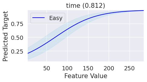
The partial dependence plot for target class 1 shows a negative relationship with feature time, indicating that as the follow-up time increases, the probability of death decreases. This is consistent with the correlation matrix, where time was negatively correlated with the target variable. Following, we can observe positive relationship the class 0 and the feature time, indicating that as the follow-up time increases, the probability of survival increases.

The monotonic behaviour of the partial dependence plot suggests that the model is ease to interpret, as shown but the XAI ease score metric.

# class 0
class_index = 0
plot_partial_dependence(partial_dependencies, ranked_importances, figsize=(5, 3), class_idx=class_index)

Surrogate metrics

from holisticai.utils import BinaryClassificationProxy
from holisticai.utils.feature_importances import compute_surrogate_feature_importance
from holisticai.inspection import compute_partial_dependence

proxy = BinaryClassificationProxy(predict=model.predict, predict_proba=model.predict_proba, classes=model.classes_)

importances  = compute_surrogate_feature_importance(X=train['X'], y=train['y'], proxy=proxy, importance_type='standard')

ranked_importances = importances.top_alpha(0.8)

partial_dependencies = compute_partial_dependence(train['X'], features=ranked_importances.feature_names, proxy=proxy)

conditional_importances  = compute_surrogate_feature_importance(X=train['X'], y=train['y'], proxy=proxy, importance_type='conditional')

y_surrogate = importances.extra_attrs['surrogate'].predict(test['X'])

y_pred = proxy.predict(test['X'])

from holisticai.explainability.metrics import surrogate_accuracy_score

surrogate_accuracy_score(y_pred, y_surrogate)

0.9166666666666666

from holisticai.explainability.metrics import classification_explainability_metrics

classification_explainability_metrics(importances, partial_dependencies, conditional_importances, test['X'], y_pred)

	value	reference
metric
Alpha Importance Score	0.100000	0.0
XAI Ease Score	1.000000	1.0
Position Parity	0.500000	1.0
Rank Alignment	0.500000	1.0
Spread Ratio	0.196356	0.0
Spread Divergence	0.230898	0.0
Surrogate Accuracy Score	0.916667	1.0

For surrogate, the interpretation of metric scores is similar to the permutation feature importance. But, we can plot the surrogate model to visualize the relationship between the features and the predicted outcome.

from holisticai.explainability.plots import plot_surrogate

plot_surrogate(importances)

<Axes: >

plot_feature_importance(importances, top_n=10)

<Axes: title={'center': 'Feature Importance'}, xlabel='Importance', ylabel='Features'>

class_index = 0
plot_partial_dependence(partial_dependencies, ranked_importances, figsize=(5, 3), class_idx=class_index)

LIME metrics

from holisticai.utils import BinaryClassificationProxy
from holisticai.utils.feature_importances import compute_lime_feature_importance
from holisticai.inspection import compute_partial_dependence

proxy = BinaryClassificationProxy(predict=model.predict, predict_proba=model.predict_proba, classes=model.classes_)

local_importances = compute_lime_feature_importance(X=train['X'], y=train['y'], proxy=proxy)

importances = local_importances.to_global()

ranked_importances = importances.top_alpha(0.8)

partial_dependencies = compute_partial_dependence(train['X'], features=ranked_importances.feature_names, proxy=proxy)

from holisticai.explainability.metrics import feature_stability

feature_stability(local_importances)

np.float64(0.8804413323983704)

The metrics used to evaluate the feature importance indicates that:

• Alpha importance score: a rasonable number of features have high importance values, suggesting a more even distribution of feature importance.

• XAI ease score: simple, linear relationship between the feature and the predicted outcome. These curves are easy to interpret.

• Position parity: low consistency in the order of feature importance, suggesting variability in model behavior across different groups.

• Rank alignment: low overlap in the top-k feature importance rankings, suggesting variability in the model’s feature importance across different groups.

• Spread ratio: distribution of feature importance is far from uniform, suggesting that the model relies on fewer, more significant features. This implies higher interpretability.

• Feature stability: the importance of features is consistent across different features, making the model more interpretable and reliable.

• Data stability: the importance of features is consistent across different instances, making the model more interpretable and reliable.

from holisticai.explainability.metrics import classification_explainability_metrics

classification_explainability_metrics(importances, partial_dependencies, conditional_importances, local_importances=local_importances)

	value	reference
metric
Alpha Importance Score	0.600000	0.0
XAI Ease Score	1.000000	1.0
Position Parity	0.120833	1.0
Rank Alignment	0.261111	1.0
Spread Ratio	0.913433	0.0
Spread Divergence	0.715095	0.0
Feature Stability	0.880441	1.0

plot_feature_importance(importances, top_n=10)

<Axes: title={'center': 'Feature Importance'}, xlabel='Importance', ylabel='Features'>

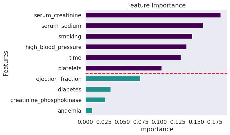
We can observe that the importances in the LIME model are not concentrated in a few features. The top-10 features show serum_sodium, time, high blood pressure, platelets, and smoking as the most important features. This is different from the permutation and surrogate feature importance, which showed time and ejection fraction as the most important features.

class_index = 1 #1
plot_partial_dependence(partial_dependencies, ranked_importances, subplots=(2,3), figsize=(12, 7), class_idx=class_index)

Partial dependence plot show that the model has a linear relationship between the feature and the predicted outcome. This indicates that the model is easy to interpret and understand.

SHAP metrics

from holisticai.utils import BinaryClassificationProxy
from holisticai.utils.feature_importances import compute_shap_feature_importance
from holisticai.inspection import compute_partial_dependence

proxy = BinaryClassificationProxy(predict=model.predict, predict_proba=model.predict_proba, classes=model.classes_)

local_importances = compute_shap_feature_importance(X=train['X'], proxy=proxy)

importances = local_importances.to_global()

ranked_importances = importances.top_alpha(0.8)

partial_dependencies = compute_partial_dependence(train['X'], features=ranked_importances.feature_names, proxy=proxy)

from holisticai.explainability.metrics import classification_explainability_metrics

classification_explainability_metrics(importances, partial_dependencies, conditional_importances, local_importances=local_importances)

	value	reference
metric
Alpha Importance Score	0.200000	0.0
XAI Ease Score	1.000000	1.0
Position Parity	0.375000	1.0
Rank Alignment	0.625000	1.0
Spread Ratio	0.393863	0.0
Spread Divergence	0.310986	0.0
Feature Stability	0.933345	1.0

The metrics used to evaluate the feature importance based on SHAP values is close to the LIME, except for the spread ratio. The spread ratio is lower for SHAP.

from holisticai.explainability.metrics import feature_stability

feature_stability(local_importances)

np.float64(0.9333448553882717)

plot_feature_importance(importances)

<Axes: title={'center': 'Feature Importance'}, xlabel='Importance', ylabel='Features'>

By analyzing the SHAP summary plot, we can observe that the most important features are time and ejection fraction, which are consistent with the permutation feature importance and surrogate importance.

class_index = 1 #1
plot_partial_dependence(partial_dependencies, ranked_importances, class_idx=class_index)

Partial dependence plot also show that the model has a linear relationship between the feature and the predicted outcome. This indicates that the model is easy to interpret and understand.

Summary

This case study explored the explainability of a Logistic Regression model trained to predict the survival of heart failure patients. We used a dataset from the UCI Repository, featuring 299 patient records with 10 clinical features.

The analysis revealed that “time” (follow-up period) and “ejection fraction” were identified as the most influential features for predicting survival outcomes, consistently across permutation feature importance, surrogate model analysis, and SHAP metrics. This finding aligns with clinical understanding, where longer follow-up periods allow for better observation of disease progression and the ejection fraction directly reflects the heart’s pumping efficiency.

The global explainability metrics highlighted the model’s overall simplicity and interpretability. The high XAI ease score, position parity, and rank alignment suggest a straightforward relationship between features and outcomes and consistent model behavior across different patient subgroups. The relatively high spread ratio reinforces this interpretability by indicating that the model primarily relies on a few, highly significant features. While LIME metrics also highlighted the model’s simplicity, they pointed to potential variability in feature importance across different subgroups and individual instances. This observation suggests the need for further investigation and potentially, model refinement to ensure consistent and equitable predictions for all patients.

This case study demonstrates the value of explainability metrics in healthcare applications of machine learning. Understanding the model’s reasoning process not only strengthens trust in its predictions but also provides valuable insights into the clinical factors driving survival outcomes for heart failure patients.