Bias Mitigation with Plugin Estimator and Calibrator

This tutorial demonstrates how to implement the “Plugin Estimator and Calibrator” postprocessing method to enhance fairness in regression models using the holisticai library.

• Traditional implementation

• Pipeline implementation

First, install the holisticai package if you haven’t already:

!pip install holisticai[all]

Then, import the necessary libraries.

import numpy as np
from sklearn.linear_model import LinearRegression
from sklearn.metrics import mean_squared_error
from holisticai.datasets import load_dataset
from holisticai.bias.mitigation import PluginEstimationAndCalibration
from holisticai.bias.metrics import regression_bias_metrics

np.random.seed(0)
import warnings
warnings.filterwarnings("ignore")

Load the proprocessed “Communities and Crime” dataset.

dataset = load_dataset('us_crime', protected_attribute="race")

dataset

[-] [Dataset]

Instances: 1993

Features: X , y , p_attrs , group_a , group_b

Metadata: race: {'group_a': 'racePctWhite>0.5', 'group_b': 'racePctWhite<=0.5'}

dataset['y'].shape

(1993,)

Now that we have a clean dataset we can start defining the protected groups and the training and testing sets.

3. Data analysis

Since this function already return the protected groups, we can start with the data analysis step. In this step, we will analyze the distribution of the data of the protected groups by using the group_pie_plot function. This function will plot the distribution of the data of the protected groups in a pie chart.

from holisticai.bias.plots import group_pie_plot

group_pie_plot(dataset['group_a'])

<Axes: >

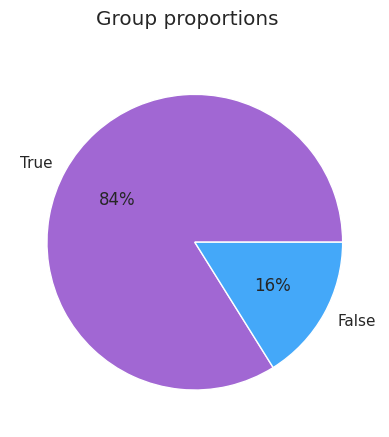
This graph show us that the proportion of white people (labelled as True) is very high compared to the remain races.

Let’s plot the columns with the highest correlations with respect to the target variable. To do this, we will use the correlation_matrix_plot function.

from holisticai.datasets.plots import correlation_matrix_plot

correlation_matrix_plot(dataset, features=['X'], target_feature="y", n_features=10)

<Axes: title={'center': 'Correlation matrix'}>

To obtain properly values with the mitigator, we will scale the objective column:

from sklearn.preprocessing import StandardScaler
import pandas as pd

scaler = StandardScaler()
y = scaler.fit_transform(dataset['y'].values.reshape(-1, 1))
y = np.squeeze(y)

# Convert the numpy array to a pandas Series
dataset['y_norm'] = pd.Series(y)

# Concatenate the series to the dataset
#dataset = dataset.map(lambda x: {'y_norm': y_series})

dataset = dataset.train_test_split(test_size=0.2, random_state=0)

train_data = dataset['train']
test_data = dataset['test']

model = LinearRegression()

model.fit(train_data['X'], train_data['y_norm'])
y_pred = model.predict(test_data['X'])

df = regression_bias_metrics(
    test_data['group_a'],
    test_data['group_b'],
    y_pred,
    test_data['y_norm'],
    metric_type='both'
)
df

	Value	Reference
Metric
Disparate Impact Q90	0.019666	1
Disparate Impact Q80	0.117994	1
Disparate Impact Q50	0.412979	1
Statistical Parity Q50	-0.705605	0
No Disparate Impact Level	-0.777897	-
Average Score Difference	-1.604353	0
Average Score Ratio	-0.235742	1
Z Score Difference	-2.750267	0
Max Statistical Parity	0.767257	0
Statistical Parity AUC	0.452860	0
RMSE Ratio	0.614069	1
RMSE Ratio Q80	0.966421	1
MAE Ratio	0.486594	1
MAE Ratio Q80	0.937572	1
Correlation Difference	0.002428	0

Bias Mitigation

Traditional Implementation

We will implement the “Plugin estimator and calibrator” method, an post-processing technique to mitigate bias in the regression model.

model = LinearRegression()

model.fit(train_data['X'], train_data['y_norm'])
y_pred = model.predict(train_data['X'])

post_processer = PluginEstimationAndCalibration()
post_processer.fit_transform(y_pred, train_data['group_a'], train_data['group_b'])
post_processer

[-] [PluginEstimationAndCalibration]

PluginEstimationAndCalibration()

---

Type: Bias Mitigation Postprocessing

y_pred = model.predict(test_data['X'])

y_pred = post_processer.transform(y_pred, test_data['group_a'], test_data['group_b'])['y_pred']

df = regression_bias_metrics(
    test_data['group_a'],
    test_data['group_b'],
    y_pred,
    test_data['y_norm'],
    metric_type='both'
)
df

	Value	Reference
Metric
Disparate Impact Q90	0.427729	1
Disparate Impact Q80	0.766962	1
Disparate Impact Q50	1.000000	1
Statistical Parity Q50	-0.058260	0
No Disparate Impact Level	0.375000	-
Average Score Difference	-0.034691	0
Average Score Ratio	0.846290	1
Z Score Difference	-0.108646	0
Max Statistical Parity	0.239676	0
Statistical Parity AUC	0.052348	0
RMSE Ratio	0.486046	1
RMSE Ratio Q80	0.435285	1
MAE Ratio	0.537228	1
MAE Ratio Q80	0.382873	1
Correlation Difference	0.167386	0

pec_rmse = mean_squared_error(test_data['y_norm'], y_pred, squared=False)
print("RMS error: {}".format(pec_rmse))

RMS error: 0.9225356257728464

Pipeline Implementation

Implementing the method using the pipeline.

from holisticai.pipeline import Pipeline

model = LinearRegression()
pipeline = Pipeline(
    steps=[
        ("model", model),
        ("bm_postprocessing", PluginEstimationAndCalibration()),
    ]
)

fit_params = {
    "bm__group_a": train_data['group_a'],
    "bm__group_b": train_data['group_b']
}

pipeline.fit(train_data['X'], train_data['y_norm'], **fit_params)
pipeline

[-] [Pipeline]

[-] model [LinearRegression]

LinearRegression(fit_intercept=.fitwrapper at 0x7ff774c725c0>, copy_X=True, n_jobs=None, positive=False, ...)

[-] bm_postprocessing [PluginEstimationAndCalibration]

PluginEstimationAndCalibration()

predict_params = {
    "bm__group_a": test_data['group_a'],
    "bm__group_b": test_data['group_b'],
}
y_pred_pipeline = pipeline.predict(test_data['X'], **predict_params)
df_pipeline = regression_bias_metrics(
    test_data['group_a'],
    test_data['group_b'],
    y_pred,
    test_data['y_norm'],
    metric_type='both'
)
df_pipeline

	Value	Reference
Metric
Disparate Impact Q90	0.427729	1
Disparate Impact Q80	0.766962	1
Disparate Impact Q50	1.000000	1
Statistical Parity Q50	-0.058260	0
No Disparate Impact Level	0.375000	-
Average Score Difference	-0.034691	0
Average Score Ratio	0.846290	1
Z Score Difference	-0.108646	0
Max Statistical Parity	0.239676	0
Statistical Parity AUC	0.052348	0
RMSE Ratio	0.486046	1
RMSE Ratio Q80	0.435285	1
MAE Ratio	0.537228	1
MAE Ratio Q80	0.382873	1
Correlation Difference	0.167386	0

pipeline_rmse = mean_squared_error(test_data['y_norm'], y_pred_pipeline, squared=False)
print("Pipeline RMSE: {}".format(pipeline_rmse))

Pipeline RMSE: 0.9225356257728464