Measuring Bias in multiclass classification

This tutorial will explain how to measure bias in a multiclass classification task using the holisticai library. We will introduce here some of the functions that can help study algorithmic bias.

The sections are organised as follows :

1. Load the data : we load the student dataset as a pandas DataFrame

2. Data Exploration : some preliminary analysis of the data

3. Train a Model : we train a model (sklearn)

4. Measure Bias : we compute a few bias metrics, and comment on their meaning

Load the data

First of all, we need to import the required packages to perform our bias analysis and mitigation. You will need to have the holisticai package installed on your system, remember that you can install it by running:

!pip install holisticai[all]

# Imports
import numpy as np
import pandas as pd
import warnings
warnings.filterwarnings("ignore")

The student dataset can be easily

from holisticai.datasets import load_dataset

dataset = load_dataset('student_multiclass', preprocessed=True)
dataset

[-] [Dataset]

Instances: 395

Features: X , y , p_attrs

Data Exploration

dataset['p_attrs']

	sex	address	Mjob	Fjob
0	'F'	'U'	'at_home'	'teacher'
1	'F'	'U'	'at_home'	'other'
2	'F'	'U'	'at_home'	'other'
3	'F'	'U'	'health'	'services'
4	'F'	'U'	'other'	'other'
...	...	...	...	...
390	'M'	'U'	'services'	'services'
391	'M'	'U'	'services'	'services'
392	'M'	'R'	'other'	'other'
393	'M'	'R'	'services'	'other'
394	'M'	'U'	'other'	'at_home'

395 rows × 4 columns

from holisticai.bias.plots import group_pie_plot
from holisticai.bias.plots import histogram_plot
from holisticai.bias.plots import frequency_matrix_plot
from holisticai.bias.plots import frequency_plot
import matplotlib.pyplot as plt

fig,axs = plt.subplots(1,4, figsize=(25,5))
p_attrs = dataset['p_attrs']
group_pie_plot(p_attrs['sex'], ax=axs[0])
group_pie_plot(p_attrs['sex'], ax=axs[1])
histogram_plot(dataset['y'], p_attr=p_attrs['sex'], ax=axs[2])
frequency_matrix_plot(p_attrs['sex'], dataset['y'], normalize='group', ax=axs[3])

<Axes: title={'center': 'Frequency matrix plot'}, xlabel='Class', ylabel='Group'>

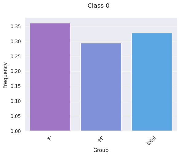
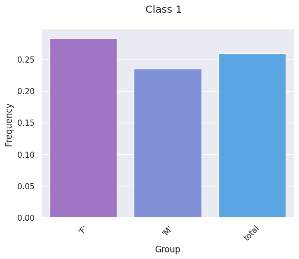
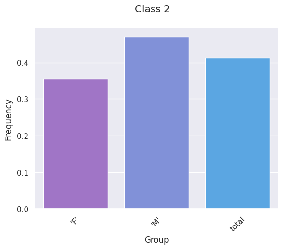
frequency_plot(dataset['p_attrs']['sex'], dataset['y'])

Train a model

datasets = dataset.train_test_split(test_size=0.3)
datasets

[-] [DatasetDict]

[-] train [Dataset]

Instances: 276

Features: X , y , p_attrs

[-] test [Dataset]

Instances: 119

Features: X , y , p_attrs

from sklearn.ensemble import RandomForestClassifier

# Train a simple Random Forest Classifier
x_train = datasets['train']['X']
y_train = datasets['train']['y']

model = RandomForestClassifier(random_state=111)
model.fit(x_train, y_train)

# Predict values
x_test = datasets['test']['X']
y_test = datasets['test']['y']
p_attr_test = datasets['test']['p_attrs']['sex']
y_pred = model.predict(x_test)

from holisticai.bias.metrics import confusion_matrix
from sklearn.metrics import precision_score, recall_score, accuracy_score

confusion_matrix(y_pred, y_test)

	0	1	2
0	16.0	13.0	9.0
1	4.0	2.0	5.0
2	12.0	18.0	40.0

# evaluate
print (accuracy_score(y_test, y_pred))
print (precision_score(y_test, y_pred, average=None))
print (recall_score(y_test, y_pred, average=None))

0.48739495798319327
[0.42105263 0.18181818 0.57142857]
[0.5        0.06060606 0.74074074]

Measure bias

from holisticai.bias.plots import frequency_matrix_plot
from holisticai.bias.plots import frequency_plot

y_pred = model.predict(x_test)   # multiclass prediction vector                                                 # multiclass label vector

frequency_matrix_plot(p_attr_test, y_pred, normalize='group')

<Axes: title={'center': 'Frequency matrix plot'}, xlabel='Class', ylabel='Group'>

Using the above plot, we observe unfairness by looking at differences over columns. For instance we look at the class 1.0, and observe how the ‘health’ group has a much higher probability of being within it.

frequency_plot(p_attr_test, y_pred)

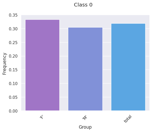
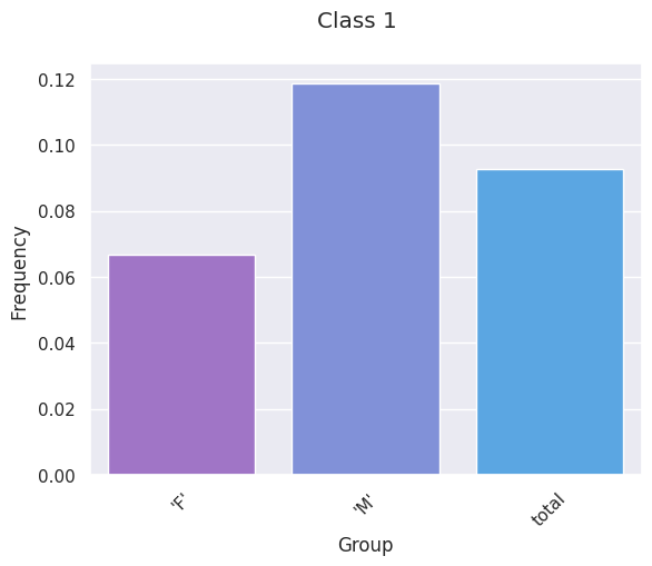
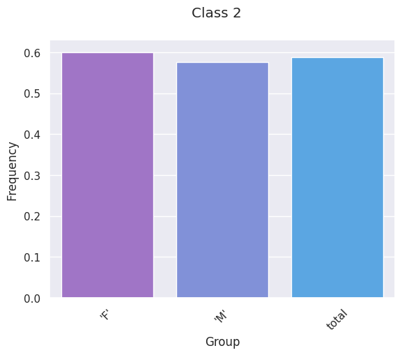
This is the same data as the previous plot, but displayed in a different way.

Let’s compute a few bias metrics. We have generalised versions of ‘1d’ bias metrics. For instance multiclass statistical parity.

from holisticai.bias.metrics import multiclass_statistical_parity

multiclass_statistical_parity(
    p_attr_test, y_pred, groups=None, classes=None, aggregation_fun="mean"
)

np.float64(0.051977401129943465)

We now compute statistical parity, generalized for the multiclass case. We aggregate by taking the average multilabel statistical parity over all possible group pairs (aggregation_fun="mean"). As in the 1d case, the suggested accepted range is (-0.1, 0.1).

multiclass_statistical_parity(
    p_attr_test, y_pred, groups=None, classes=None, aggregation_fun="max"
)

np.float64(0.051977401129943465)

Alternatively, we could aggregate by taking the maximum (aggregation_fun="max") over all possible group pairs. As expected, the maximum statistical parity is higher in this case.

We can try another bias metric, for instace multiclass_equality_of_opp is the multidimensional version of the 1d equal opportunity metric.

from holisticai.bias.metrics import multiclass_equality_of_opp

multiclass_equality_of_opp(
    p_attr_test, y_pred, y_test, groups=None, classes=None, aggregation_fun="mean"
)

np.float64(0.3224740773502383)

multiclass_equality_of_opp(
    p_attr_test, y_pred, y_test, groups=None, classes=None, aggregation_fun="max"
)

np.float64(0.3224740773502383)

from holisticai.bias.metrics import multiclass_bias_metrics
multiclass_bias_metrics(p_attr_test, y_pred, y_test, metric_type='both')

	Value	Reference
Metric
Max Multiclass Statistical Parity	0.051977	0
Mean Multiclass Statistical Parity	0.051977	0
Max Multiclass Equality of Opportunity	0.322474	0
Max Multiclass Average Odds	0.076275	0
Max Multiclass True Positive Difference	0.172115	0
Mean Multiclass Equality of Opportunity	0.322474	0
Mean Multiclass Average Odds	0.076275	0
Mean Multiclass True Positive Difference	0.172115	0